|
Oregon IPM Center at OSU
US Degree-Day Mapping Calculator and Publisher
Documentation - Version 4.0+
These degree-day maps are custom made according to inputs you specify. They are derived from accumulated and near real-time temperatures from AGRIMET, Hydromet, National Weather Service, RAWS, SNOTEL, CWOP and certain grower networks, PRISM temperature maps, and degree-day calculations from up to 12,000+ sites in the coterminous USA. In addition, historical average data from thousands of stations are available for Historical Average DD Maps. Making a degree-day map is now a 2-step process: 1) Select settings and click MAKE MAP (be prepared to wait up to several minutes), and 2) Click GRASSLinks "GO" for interactive GIS interface to degree-day maps. An optional third step is to download the resulting ascii GIS data with limited metadata, ready to unzip and load into a compatible GIS (tested with ESRI ARCGIS and GRASS GIS 5.x and 6.x).
Back to US Degree-day Mapping Calculator.
(NOTE: if another user is currently using the mapping calculator, your request will fail and you should: try the other server from our home page, or wait a minute or two and try again!)
Version 4.0 New Features
- Updated PRISM maps (800m resolution)
- Support for subregions in most states
- Ability to download GIS data
Purpose
- The purpose of this calculator is to allow free access to technology that enables the making of degree-day maps of states and regions in the US, for pest management decision making support. We have combined real-time weather data, a degree-day calculator, PRISM climate mapping, GIS analysis, and online map publishing capabilities into a web-based tool. Also, since 2005, this tool has been configured to work with handheld PDAs and Cellphones in the field (for this we recommend "tiny" for map size). Please do not use or advertise this tool if you have no real interest in pest management or crop production. This resource is limited and may not work well if too many people access it at the same time.
Brief Documentation of DD Map Construction
Ths system consists of an online degree-day mapping calculator, usmapmaker.pl, (Coop 2010) which uses publicly available weather data and PRISM climate maps (Daly et al. 2002) to produce degree-day maps. The system uses a method in common use, termed 'climatologically aided interpolation' (CAI) (Willmott and Robeson 1995), and follows these steps:
1) After the user enters thresholds, calculation method, the range of dates for calculation, and mapping options, they click on the "Calc" button,
2) The web/GIS server receives user inputs and begins by starting a GIS session in GRASS (Neteler and Mitasova 2008),
3) The GIS first calculates PRISM-only based degree-days using PRISM monthly average maximum and minimum temperature GIS raster maplayers,
4) All site data from public weather networks (including METAR, RAWS, APRSWXNET, AGRIMET, SNOTEL, and many others) are processed using a site-only degree-day calculator,
5) The more accurate site-based degree-days are then subtracted from PRISM-only degree-day estimates at the same locations as sites,
6) These differences are then spatially interpolated using inverse distance weighted (IDW) interpolation,
7) This difference raster layer is then added as a correction layer to the PRISM-only maplayer to produce the CAI-corrected map.
8) Additional reference layers (roads, political boundaries, etc.) are added and the map is converted to a web-compatible graphic format and returned to the user.
This degree-day mapping calculator has been available as a coterminous-US web-based tool since 2005 and for Oregon since 2000.
9) Results are available both as web image files (PNG, GIF, and JPG formats), and as GIS Arc Ascii format, allowing import by many GIS programs for further processing and customized mapmaking.
Citing this application:
No formal peer reviewed publications currently document this product. We suggest you cite it either directly as a website or via this documentation page:
Cite this documentation page as:
Coop, L. B. 2010. U. S. degree-day mapping calculator and publisher - Documentation Version 4.0. Oregon State University Integrated Plant Protection Center Web Site Publication E.10-04-2: http://uspest.org/wea/mapmkrdoc.html
Cite the application as:
Coop, L. B. 2010. U. S. degree-day mapping calculator. Version 4.0. Oregon State University Integrated Plant Protection
Center Web Site Publication E.10-04-1: http://uspest.org/cgi-bin/usmapmaker.pl
Other related citations for this product:
Daly, C., W. P. Gibson, G.H. Taylor, G. L. Johnson, P. Pasteris. 2002. A knowledge-based approach to the statistical mapping of climate. Climate Research, 22:99-113.
Neteler, M. and H. Mitasova, 2008. Open Source GIS: A GRASS GIS Approach. Third Edition.
The International Series in Engineering and Computer Science: Volume 773. 406 pages, Springer, New York
Willmott, C. J., and S. M. Robeson, 1995: Climatologically aided interpolation (CAI) of terrestrial air temperature. Int. J. Climatol., 15:221–229.
Guidelines for using the DD Map Calculator
- Learn degree-day basics and specifics on your model of interest - Please read the information provided on this page. In addition, you can learn about using degree-days and models from most of the other web pages at our home page (IPM Pest and Plant Disease Models and Forecasting). In particular, try the IPM degree-days and models - Frequently Asked Questions (FAQ) page for basics. Also, take a look at IPM pages developed at UC Davis. One page provides a good technical introduction to degree-day and phenology modeling concepts. A comprehensive library of degree-day model summaries from UC Davis is at http://www.ipm.ucdavis.edu/MODELS/index.html. At this website, you may check available models on the from this list. To see a model summary, click on the model abbreviation (fourth column in table) to display model parameters to use as inputs to the mapping calculator. For example, for codling moth (2008 model), you get a summary table such as this:
========MODEL INPUTS========
Model species:	 	WSU codling moth model 2008 [apple & pear]
Type:			 	insect
Model source:	 	Jones, Doerr & Brunner 2008
Calculation method:	single sine curve
Lower threshold:		50 degrees Fahrenheit
Upper threshold:		88 degrees Fahrenheit
Directions for starting/BIOFIX:	 Calendar date Jan 1
Model validation status: actively undergoing evaluation
Region of known use:     support for use in WA only
========EVENTS TABLE========
1.  175 DDs after Jan 1: Estimated first catch in Pheromone traps (biofix)
2.  395 DDs after Jan 1: 1ST GEN.: 1% EGG HATCH
3.  830 DDs after Jan 1: 1ST GEN:50% EGG HATCH, 97% MOTH FLIGHT
========================
From this table, in the usmapmaker.pl program, enter 50 as the lower temperature threshold, 88 as the upper threshold, single sine as the calculation type, and Jan 1 as the starting date. Once a map is calculated, using the default Query mode in the GRASSLinks display, locations that result in degree-days greater than a given event are expected to have already happened. For example, if a location is queried and returns 180 DDs, then first catch is expected to have already occurred there (>175 DDs). More details continue below:
- Basic usage - Before you begin, have ready all required input parameters for degree-day mapmaking. Enter values where appropriate in the form (options detailed below). Next enter mapping options such as region and subregion. Click on "MAKE MAP" and be prepared to wait 20 seconds to several minutes depending on your settings. Clicking "GO" will start a GRASSLinks session to view and interact with the map, plus a new window will open to display a legend showing cumulative degree-days and associated colors that should help you interpret the map. In GRASSLinks, you may zoom, re-center, and query site-specific degree-days. Using the legend, if a given location has a color that matches the color in the legend, then you have a prediction that the event has already or is now occuring. Also, if you click in the map with the "Query" option, the query results will include the degree-days for the location you clicked on. The query returns a link to a site DD calculator for the nearest station. Change DD calc settings to match your map, click "calc", and compare the map results to the site calculator.
- Process time - This mapping calculator runs on an "Intel/AMD" based server (currently a dual quad-Xeon 3.3 GHz HP ProLiant DL380 G5 using CENTOS 5.x), and requires between 20-300 seconds or more to compute your map, depending options. During processing, watch the status bar at the bottom of your browser (if enabled in browser settings). On some browsers, an animated GIF of the USA will display the steps used in DD mapmaking. Once finished, a GRASSLinks "GO" button will appear. Click on this to enter the interactive GIS interface. Do not submit "Make Map" twice before the first map is returned to you.
- Computing resource use - Note that only one concurrent user of the mapmaking calculator is allowed per server (currently 2 servers are available). Once the map is constructed, the GRASSLinks interface should allow access to it for several hours (and other users can construct maps during this time). If someone else has the mapmaker tied up, the hourglass should quickly change back to your normal mouse cursor, and you will not see the correct map (if any). When this occurs, check your parameters and try again. To speed up processing, try selecting the smaller image sizes, a subregion (except smaller New England states), small mapsize, and "original" resolution.
- Resolution - The default resolution of most maps is 800 x 800m cells (since vers. 4.0 was release Mar 1, 2010; full coterminous-US and region maps are lower res.), which derives from PRISM base map resolution. We smooth the data so that it appears finer than that, but keep in mind that topographic features smaller than about 800 x 800m will not likely be included. The "enhanced" resolution option currently adds little improvement to the maps (since updating to vers. 4). In some situations (long periods of time over mountainous terrain) it may be worth the extra processing time. You can obtain the exact resolution settings from the zipped metadata file.
- Using GIS data downloads - Since Vers. 4.0, you may download the zipped GIS ascii data and basic metadata (ascii XXX.meta.txt file) for incorporation into your GIS. Just click on the "zipped" link below the "GO" button and save to your computer. This is zipped ESRI ARC ascii grid data (unprojected lat-long), which experienced GIS users should already be familiar with. The data are integers (degree-days Fahrenheit; Celsius not available, but simply divide the data by 1.8 to obtain Celsius DDs). Basic metadata includes user input settings, how to give credit to this website if used for a product or service, resolution information, and color table info. Note color table information is in GRASS GIS (5.x-6.x) format. You can perhaps use this as a guideline in building your own color table. Also compare our GRASSLinks display of the data and legend to your GIS for verification.
- Credits - Please acknowledge any data or outputs incorporated into your products or services. A basic credit would look like this:
- Degree-day GIS Data Source: provided by Oregon State University, OIPMC, http://uspest.org/wea,
- with support from USDA NIFA NPDN, www.npdn.org.
- Public weather data provided in part by U. Utah-Mesowest;
- PRISM climate data by OSU PRISM Group.
Calculator Options
- Lower temperature threshold - This is the theoretical temperature below which development does not occur. Only integers between 10-60 degrees Fahrenheit are currently allowed by this program.
- Upper temperature threshold - This is the theoretical temperature above which development does not occur. Only integers between 32-112 degrees Fahrenheit are currently allowed by this program. The default, 130, indicates that no upper threshold is used. Only a horizontal upper cutoff method is used. The vertical upper cutoff method has not been implemented in this program.
- Calculation type - Degree-days are approximations of the temperature integrated over a time interval. Since we use only daily maximum and minimum temperatures to calculate degree-days, we have developed several methods to approximate actual degree-days. These vary in complexity and accuracy. In general, use the method recommended by the person who developed a given degree-day model. The triangle and sine methods are fairly accurate and can usually be substituted for actual or hourly-based degree-days as a reasonable and expedient substitute. In any formulae given below, Tlow is used to refer to the lower threshold, Thi is used to refer to the upper threshold.
- simple average - This method is simple to express for cases where no upper cutoff is used: (max + min) / 2 - Tlow.
The simple average method is used for many insect, weed, and crop models. Note that for weed and crop models, this method may be referred to as "growing degree-days" (GDD). Be sure to check your sources and use the appropriate method, regardless of the naming confusion.
- growing dds - This method is used for some crop (such as corn) and weed development models. It differs from the simple average method by using substitutions. The formula is: (max + min) / 2; if the min is lower than Tlow then substitute min with Tlow; if the max is higher than Thi then substitute max with Thi.
- single triangle - This method computes the area of a triangle using todays min for the lower 2 points and todays max for the upper point, but with "clipping" where thresholds are exceeded. It was developed by Sevecherian Stern & Mueller (1977).
- double triangle - This method adds together the area of two triangles using today and tomorrow's mins for each half-day triangle, and todays max for both, again with "clipping" where thresholds are exceeded.
- single sine - This method is mathematically more complex; it fits a sine curve function between the max and min temperatures and computes the area under the curve using todays min for the lower 2 points and todays max for the upper point, but with "clipping" where thresholds are exceeded. The sine methods used here were published in: Baskerville, G. L. and P. Emin. 1969. Rapid estimation of heat accumulation from maximum and minimum temperatures. Ecology 50: 514-517.
- double sine- This method fits a sine curve function between the max and min temperatures and computes the area under the curve using today and tomorrows mins for the lower 2 points and todays max for the upper point, but with "clipping" where thresholds are exceeded.
- heating and cooling degree-days- This is a simple calculation that expects you to enter "65" as the lower temperature threshold for both heating and cooling DDs. Set the upper threshold to the default (130). Used by the power industry to estimate heating and air-conditionaing costs.
- Start date (BIOFIX) - Degree-days are reset to zero on the day before the BIOFIX date, and degree-days begin accumulating on the BIOFIX date.
- End date: - Degree-days are accumulated from the start date to the end date. The degree-day mapping program does not currently support forecasting, so normally the end date will be yesterday, or some user-specified date earlier than yesterday. If prior years data are available for the region (before 2005 data available for W. US only), then any interval between Jan 1 and Dec 31 should work. Spanning the new year is not supported, so a map of degree-days between Dec. 1 2009 and Jan 31 2010, for example, would not work. For historical 30-year average (Normals) maps, any end date is allowed. Deviations between this year and Normals (and last year DD) likewise only allow calculation to yesterdays date.
- Map type:
- current year - As of 2009-2010, we support 12,000+ stations across the coterminous USA to allow maps for any state or region.
- previous years - Note that as of 2004, we supported 1400+ stations across the western USA. Since 2005 full coterminous-US maps are allowed.
- historical average - These maps generally use 30 year average data from a smaller set of weather stations than we now have for the current year. These maps can be very useful for indicating "average" development trends and differences between locations. In some cases you should be able to make "forecasting" maps using todays date as the Start date (BIOFIX), and a future date as the end date. The "forecasted" cumulative degree-days would then represent a prediction of future degree-days that could be added to the current map and compared to models.
- deviations vs. last year - Will compute the difference between DDs this year and last, and will show this years progress relative to last year. Values are negative (indicated with a gray to black color scale) when it has been cooler than last year. Values that are warmer are shown using the same color legend used for the other degree-day maps.
- deviations vs. 30-year average - These maps are especially useful in showing this years progress relative to the historical normals. Values are negative (indicated with a gray to black color scale) when it has been cooler than the historical average. Values that are warmer are shown using the same color legend used for the other degree-day maps.
Mapping Options
- Region - This program has evolved from an Oregon-only mapmaker to (beginning 2005) allow maps of the entire coterminous 48-state US. In addition to single states you may choose to make maps of entire regions, which will be slow, and are sometimes at reduced resolutions. Maps of the full 48-state US are allowed, but at a greatly reduced resolution, due to computing constraints. Current region options include:
- US 48-state - Coterminous US; resolution restricted to ca. 2'30" (ca. 4km).
- PNW 3-state - The Pacific Northwest states of OR, WA, and ID; res. restricted to ca. 1'15" (ca. 2km).
- NW 5-state - The Northwest states of OR, WA, ID, MT, and WY (ca. 2km).
- NW 9-state - The Northwest states of OR, WA, ID, MT, and WY, plus N. CA, N. AZ, UT and CO (ca. 2km).
- W 11-state - The Western states of OR, WA, ID, MT, WY, CA, NV, UT, AZ, CO, and NM (ca. 2km).
- SW 4-state - The SW states of CA, NV, UT, and AZ (ca. 2km).
- SW 6-state - The SW states of CA, NV, UT, AZ, CO, and NM (ca. 2km).
- S 13-state - The Southern states of TX, OK, AK, LA, TN, MS, AL, NC, SC, GA, and FL (ca. 2km).
- N. Central states ND, SD, NB, KS, MN, IA, MO, WI, and IL.
- NE states ME, NH, VT, CT, RI, NY, PN, MD, and DL.
- SW Calif. Including from Santa Barbara to San Diego.
- Subregion - All states except the smaller New England states have predefined subregions representing 4 corners plus central areas. This option does not currently apply to ME, NH, VT, CT, RI, MD, and DL. For all other states, however you may select the NW, SW, NE, SE, or central portion of a single state. This will speed up mapmaking. The resolution enhancement option MAY give reasonable performance if using a subregion, otherwise it is not recommended.
- Mapsize - images 9k - 122k depending on region, size, and image type
- tiny - 300 pixels wide by 156 high. File size ca. 9k depending on region image type.
- small - 440 pixels wide by 229 high. File size ca. 16k depending on region and image type.
- regular - 600 pixels wide by 446 high. File size ca. 22k depending on region and image type.
- large - 900 pixels wide by 544 high. File size ca. 61k depending on region and image type.
- huge - 1200 pixels wide by 800 high. File size ca. 122k depending on region and image type.
- Legend - Options for different legends were added to accomodate different ranges in DD accumulations, to provide better resolution and ease of map reading. The default is "heat ramp", which stretches a fairly standard range of colors over the full range of degree-days to give a natural separation of results. After the map is constructed, the legend is opened in a separate window. Note that if you already have a second window open, which is hidden underneath the current window, then you may not see the legend until you raise it to the top of your desktop.
- Resolution - Enhanced option (not currently recommended) - This option invokes an extra step known as geographically weighted regression, to attempt to improve resolution. The process is described for DD maps here. Now (Vers. 4.0) that most DD maps are built with hi-resolution (800m) PRISM data, and are nominally smoothed to ca. 270m, this option is no longer expected to significantly improve the DD map resolution. Also this step usually doubles or triples the processing time. The option was not removed, however, because in some cases the final map can appear to reproduce elevation/terrain contours more successfully. Use with caution - try using with a state subregion, for a long time interval, and in a mountainous state, for best results. Below (Fig. 1) is an example showing how standard State/subregion resolution (800m or 30 sec) (Fig. 1c) is much better than for the 48-state US (color table adjusted) (1a) and for a large region (3 state PNW) (1b), but not much improved by using the "Enhanced Resolution" option (1d). If you zoom in on the latter two, some subtle improvements are evident from using enhanced resolution (Fig. 2). Thus, the cases where this option adds to precision and presentation quality of a DD map are probably very few.
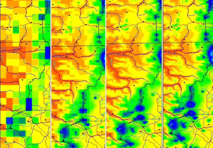
Fig. 1. Example Resolution Comparison - Oregon Central Cascades Jan 1- June 28, 2009
From left: a) US_vlo (2:30 ca. 4km), b) PNW_lo (:75 ca. 2KM) c) orig. OR (:30 ca. 800m ) d) Enhanc. Res. (:10 ca. 270m);
scale of miles: ca. 30 miles west to east, 120 miles north to south
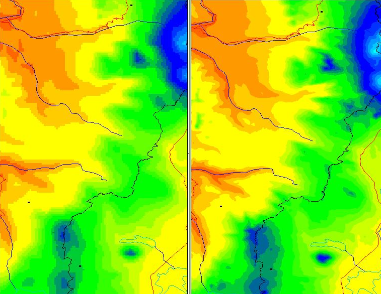
Fig. 2. Example Resolution Comparison - Oregon Central Cascades Jan 1- June 28, 2009 (closeup of Fig. 1c & 1d above)
From left: a) orig. OR (:30 ca. 800m ) b) Enhanc. Res. (:10 ca. 270m); scale of miles: ca. 25 miles west to east, 40 miles north to south
- Overlay - The default was changed to "none" (Vers. 4.0); vs. a shaded terrain layer that (if selected) is merged into the degree-day layer. This layer provides a better sense of terrain, at the cost of sometimes partially obscuring degree-day results.
Features yet to add and known bugs to be fixed
- Add ability to process maps for multiple concurrent users
- Add ability to combine forecasts with current maps
Other information:
 Older summary of methods used to create degree-day maps Older summary of methods used to create degree-day maps
[Home]
[Intro]
[Table Index]
[DD Models]
[DD MapCalc]
[Links]
This project funded in part by grants from the USDA-WRIPM and USDA-NPDN programs.
This page on-line since Dec. 9, 1998
This page updated Apr. 27, 2010
Contact Len Coop at coopl@science.oregonstate.edu if you
have any questions about this information.
|